1 Psst…we need to talk
“The secret to writing better is reading more.”
-someone
Reading aloud
Let’s practice reading R scripts with a partner.
They’ll listen to what you say and turn it into R code.
It’s like a game of telephone, but for R.
Instructions
- Find a partner.
- One of you gets to be Bert and one of you is Ernie.
- Bert will look at the first code block and tell Ernie what it does.
- Ernie will then write some code that accomplishes what Bert said.
- Then Bert can offer more clues to help.
- Try not to say the exact names of functions, like “use
filter” or “usewrite_csv” - Instead, say what you want to accomplish, like
"Drop the rows where..."or"Save the data as..."
- Try not to say the exact names of functions, like “use
Example code to read aloud
Say aloud what this code does or tries to accomplish.
⚠️ Wait to click below until you decide who’s Bert.
1. Bert’s turn to read: BIG fish
No peaking Ernie!
We’ll start by turning some fishy code into plain language.
Bert’s s only!
2. Ernie’s turn to read: Sleepy sheep 🐑🐑🐑
Ernie’s s only!
3. Charades! Act it out
Instead of saying what the code does aloud, act out what the code does without speaking at ALL.
Ask Barbara very nicely to go first.
Barbara’s s only!
2 Pipe things together: A %>% B
Wishing you could type the name of the data less often?
You can with the pipe!
Use the %>% to chain functions together and make our scripts more streamlined and easier to read. When reading code with the %>% you can read it as and then.
For example
puppy
%>%runs_outside%>%rolls_in_mud%>%barks_joyfully(times = 3)
Can be read as
There is a puppy, it runs outside
And thenrolls in the mudAnd thenbarks joyfully 3 times.”
The %>% helps:
1. Eliminate nested parentheses
Let’s say you have 3 numbers. Your analysis requires that you take the sum of them, then take the log of that result, and then round the final outcome.
Without the pipe
The code above is dense and we need to read it backwards from right to left to understand the order of operations. The pipe on the other hand allows us to read the code from left to right.
2. Combine processing steps into a cohesive chunk
Without the pipe
Let the %>% guide you.
3 Connect to databases
Databases and SQL
Prep
Let’s get our favorite starwars data.
#install.packages("RSQLite")
#install.packages("DBI")
library(RSQLite)
library(DBI)
library(dplyr)

people <- starwars
Create a local db
# Create a connection to a new database
# A .db file will appear in your project folder
conn <- dbConnect(RSQLite::SQLite(), "people.db")
Add our data
# Add the dataset to a table called "people_tbl"
## ERROR! This will throw an error about our data
try(dbWriteTable(conn, "people_tbl", people))

# Drop the list columns
people <- select(people, -films, -vehicles, -starships)

# Try again
try(dbWriteTable(conn, "people_tbl", people))

# List all the tables available in the database
dbListTables(conn)
Reading data
SQL
dbGetQuery(conn, "SELECT * FROM people_tbl")

# Filter the data
df <- dbGetQuery(conn, "SELECT * FROM people_tbl
                        WHERE eye_color = 'brown'")
dplyr
## # Source: table<people_tbl> [?? x 11]
## # Database: sqlite 3.39.4 [/cloud/project/content/page/people.db]
## name height mass hair_…¹ skin_…² eye_c…³ birth…⁴ sex gender homew…⁵
## <chr> <int> <dbl> <chr> <chr> <chr> <dbl> <chr> <chr> <chr>
## 1 Luke Skywa… 172 77 blond fair blue 19 male mascu… Tatooi…
## 2 C-3PO 167 75 <NA> gold yellow 112 none mascu… Tatooi…
## 3 R2-D2 96 32 <NA> white,… red 33 none mascu… Naboo
## 4 Darth Vader 202 136 none white yellow 41.9 male mascu… Tatooi…
## 5 Leia Organa 150 49 brown light brown 19 fema… femin… Aldera…
## 6 Owen Lars 178 120 brown,… light blue 52 male mascu… Tatooi…
## 7 Beru White… 165 75 brown light blue 47 fema… femin… Tatooi…
## 8 R5-D4 97 32 <NA> white,… red NA none mascu… Tatooi…
## 9 Biggs Dark… 183 84 black light brown 24 male mascu… Tatooi…
## 10 Obi-Wan Ke… 182 77 auburn… fair blue-g… 57 male mascu… Stewjon
## # … with more rows, 1 more variable: species <chr>, and abbreviated variable
## # names ¹hair_color, ²skin_color, ³eye_color, ⁴birth_year, ⁵homeworld
## # ℹ Use `print(n = ...)` to see more rows, and `colnames()` to see all variable names# Filter the data
df <- tbl(conn, "people_tbl") %>%
filter(eye_color == "brown")
# Show the SQL that *will* run, if you tell it to
show_query(df)## <SQL>
## SELECT *
## FROM `people_tbl`
## WHERE (`eye_color` = 'brown')Database parameters for the real world
driver: Specific to the type of database: Oracle, PostgreSQL, Athenaurlorhost: The web or server location to connect to
port: A 4 digit number of the port to use for communicating with the db
db: The db name
user: Your username for the db
password: Your password for the db
Woah! That is a lot to keep track of. Luckily, there are helper packages to simplify connecting to various databases. Contact your Agency’s R user group for more info.
4 Password: Is it secret, is it safe?
Using passwords in R
Not secret, not safe
Yes secret, Yes safe
Connecting to Agency databases
A live demo will begin shortly…
5 Your turn
Time to start putting what we’ve learned to use. Choose one of the paths below and use your new hard-earned R skills to explore data. When you feel ready, jump to the Grand Moff path and begin making a report for your own data.
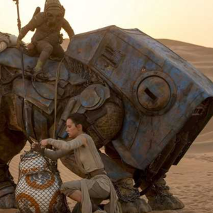
Explore the scrap and salvage economy on Jakku.
Media: solid waste
Planet: Jakku
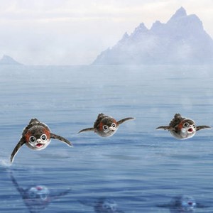
Study the effects of jet-fuel on Porg reflexes.
Media: biological
Planet: Ahch-To
Travel back to Earth and explore your own data set.
Media: all
Planet: Earth
What’s next?
Join us!
- R user groups: TidyTuesdays
- R Teams in Teams
R heroes
Online courses
- John Hopkins’ Exploratory Data Analysis
Web trainings
- RStudio Primers
- Intro to R - Cute giraffes!
- R boot camp - The Magic of ggplot2
Online books
🐱 Concatulations!
You were an excellent Data Droid! Rey and BB8 absolutely couldn’t have done it without you.
You deserve an award.
    Meowwwwww R Users!
      \
       \
        \
            |\___/|
          ==) ^Y^ (==
            \  ^  /
             )=*=(
            /     \
            |     |
           /| | | |\
           \| | |_|/\
      jgs  //_// ___/
               \_)
Return to Earth
You’re free! You can return to Earth now. Go ahead and robot frolic in the grass, enjoy the solar power, and jump in a lake. To help you fully acclimate, let’s look at some Earth data.

Study the housing habits of Earthlings. Create interactive maps showing the spatial clustering of different social characteristics of the human species.
Media: social-human
Planet: Earth