
Remember what you should do first when you start your R session? First we load the packages we will need.
#Load packages
library(readr)
library(dplyr)
library(ggplot2)
Start by reading in the data. It is a clean version of the scrap data we’ve been using.
Notice that we are including comments in the R script so that your future self can follow along and see what you did.
Read in data
clean_scrap <- read_csv("https://mn-r.netlify.com/data/starwars_scrap_jakku_clean.csv")

head(clean_scrap)
## # A tibble: 6 × 6
## items origin destination price_per_…¹ amoun…² total…³
## <chr> <chr> <chr> <dbl> <dbl> <dbl>
## 1 electrotelescope outskirts trade caravan 850. 868. 7.38e5
## 2 atmospheric thrusters cratertown niima outpost 56.2 33978. 1.91e6
## 3 bulkhead cratertown raiders 1005. 645. 6.48e5
## 4 main drive blowback town trade caravan 598. 1961. 1.17e6
## 5 flight recorder outskirts niima outpost 591. 887 5.24e5
## 6 proximity sensor outskirts raiders 1229. 7081 8.70e6
## # … with abbreviated variable names ¹price_per_ton, ²amount_tons, ³total_priceDid it load successfully? Look in your environment. You should see “clean_scrap”. There should be 6 variables and 573 rows.
Take a couple of minutes to get an overview of the data. Open and look at your data in at least two ways.
Click on the data name in the environment to open the window.
Use glimpse() to look at your data.
Show solution
#View the data
glimpse(clean_scrap)
## Rows: 573
## Columns: 6
## $ items <chr> "electrotelescope", "atmospheric thrusters", "bulkhead",…
## $ origin <chr> "outskirts", "cratertown", "cratertown", "blowback town"…
## $ destination <chr> "trade caravan", "niima outpost", "raiders", "trade cara…
## $ price_per_ton <dbl> 849.79, 56.21, 1004.83, 597.85, 590.93, 1229.03, 56.21, …
## $ amount_tons <dbl> 868.4280, 33978.1545, 644.7285, 1960.6650, 887.0000, 708…
## $ total_price <dbl> 737981.43, 1909912.06, 647842.54, 1172183.57, 524154.91,…Look at a summary of your data using summary().
Show solution
#View a summary of the data
summary(clean_scrap)
## items origin destination price_per_ton
## Length:573 Length:573 Length:573 Min. : 29.15
## Class :character Class :character Class :character 1st Qu.: 314.23
## Mode :character Mode :character Mode :character Median : 629.28
## Mean :1010.85
## 3rd Qu.:1329.05
## Max. :7211.01
## amount_tons total_price
## Min. : 0.01 Min. : 5
## 1st Qu.: 238.99 1st Qu.: 128921
## Median : 1298.00 Median : 757656
## Mean : 3724.23 Mean : 3483802
## 3rd Qu.: 4678.44 3rd Qu.: 2631778
## Max. :60116.67 Max. :83712615What if you only want to keep the items and amount_tons fields? Use select() to create a new data frame keeping only those columns and save it as an object called
select_scrap.
Show solution
select_scrap <- select(clean_scrap, items, amount_tons)Order the data frame you just created by
amount_tonsfrom highest to lowest. Which item had the highest weight?
Show solution
select_scrap <- arrange(select_scrap, desc(amount_tons))Filter your select data set to all items with an amount higher than 1000. Call the dataset ‘filter_scrap’
Show solution
filter_scrap <- filter(select_scrap, amount_tons > 1000)Add a filter to to the amount_tons > 1000 dataset. Include only “proximity sensor” and “hyperdrive”
Show solution
You will need %in%, c() and filter.
Show solution
filter_scrap <- filter(select_scrap, amount_tons > 1000,
                       items %in% c("proximity sensor", "hyperdrive"))
Use mutate() to add a column calculating the amount of pounds from the
amount_tonscolumn. Name the columnamount_pounds.
Show solution
filter_scrap <- mutate(filter_scrap, amount_pounds = amount_tons * 2000)We want to make a table of recommendations for our shopping. In our filtered dataset, we want to buy scrap if it is a
Hyperdriveand ignore it when it’s not.Use mutate() to add a column that says “buy” if the item is a
Hyperdriveand “ignore” if it’s not. Name the new columndo_this. You will need both ifelse() and mutate() for this task.
Show solution
filter_scrap <- mutate(filter_scrap, do_this = ifelse(items == "hyperdrive", "buy", "ignore"))
Let’s take a closer look at our full dataset now (clean_scrap). We want to give the Junk Boss a summary of all of this data. He hates numbers, but he likes money.
He wants to know the following things:
- The sum of all the money potentially earned by item.
- The maximum money potentially earned by item.
- The number of records of each item.
- The 35th percentile of the price by item.
_*Curious how he knows about quantiles, maybe someone told him to use this to test our abilities._
Hint:
You will need the pipe %>%, group_by(), summarise(), sum(), max(), quantile(), and n().
Hint # 2!
summary_scrap <- clean_scrap %>%
                 group_by() %>%
                 summarise()
Show solution
summary_scrap <- clean_scrap %>%
  group_by(items) %>%
  summarise(sum_price = sum(total_price),
            max_price = max(total_price),
            count_price = n(),
            price_35th = quantile(total_price, 0.35))
Oh boy, Unkar just learned about plots. What will he want next?
Now he wants a plot of the maximum total prices by item.
Try both
geom_col()andgeom_point()to see which makes a simpler plot to understand.
Show solution
ggplot(data = summary_scrap, aes(items, max_price)) +
  geom_col()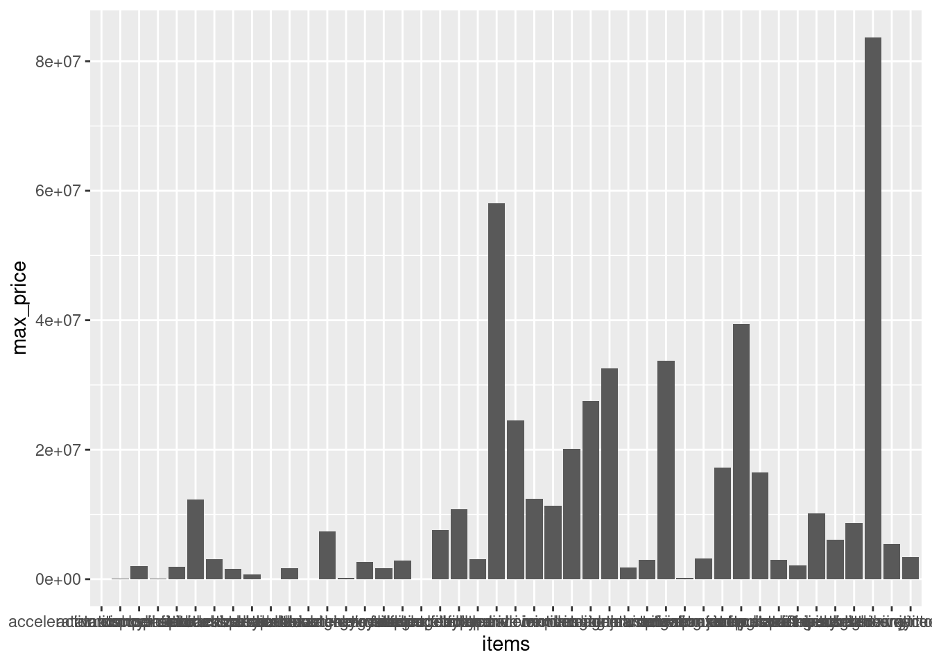
Show solution
ggplot(data = summary_scrap, aes(items, max_price)) +
  geom_point()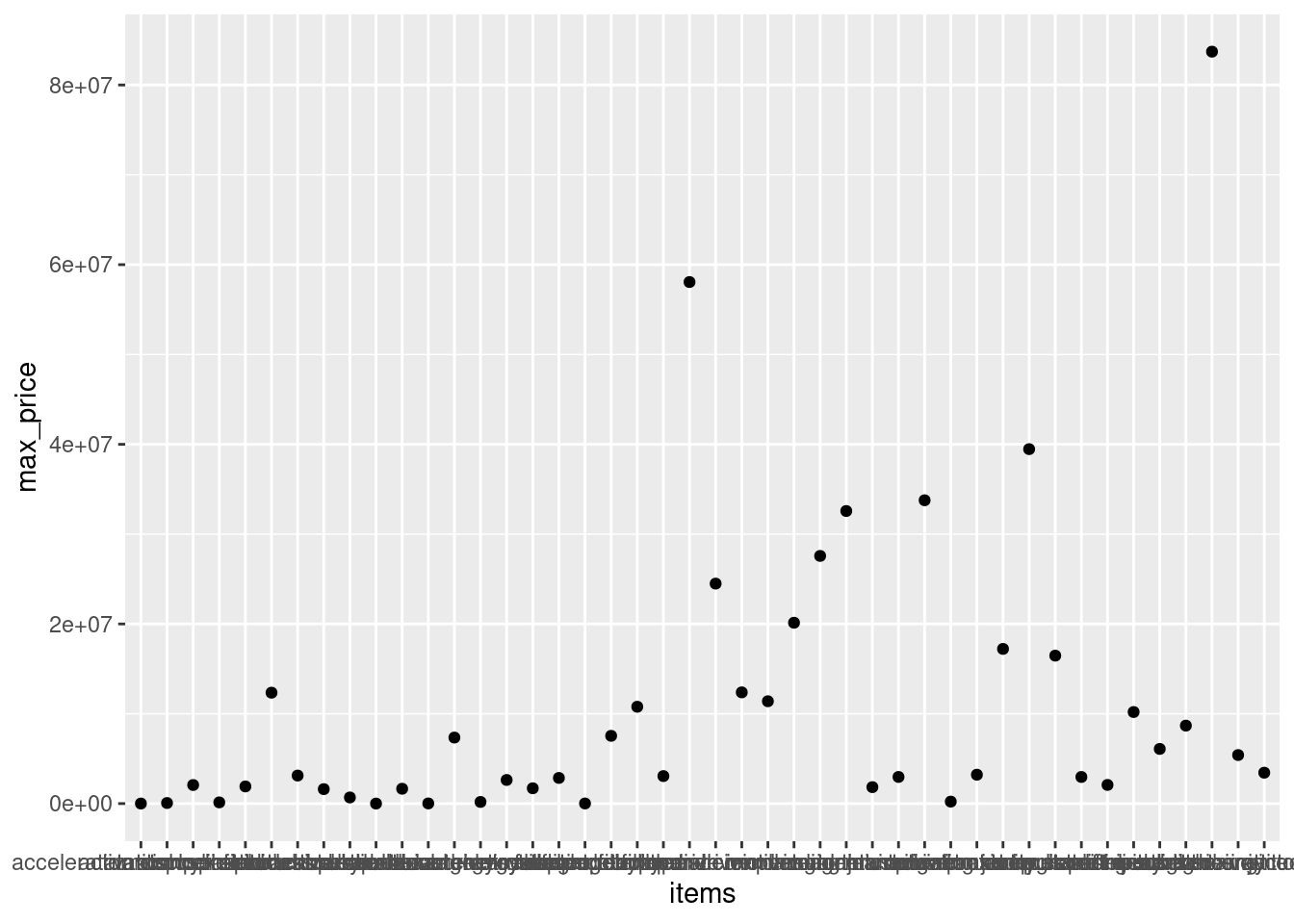
Try
coord_flip()to make the plot more readable.If you’re interested in learning more about
coord_flip(), ask R for help!?coord_flip
Show solution
ggplot(data = summary_scrap, aes(items, max_price)) +
  geom_col() +
  coord_flip()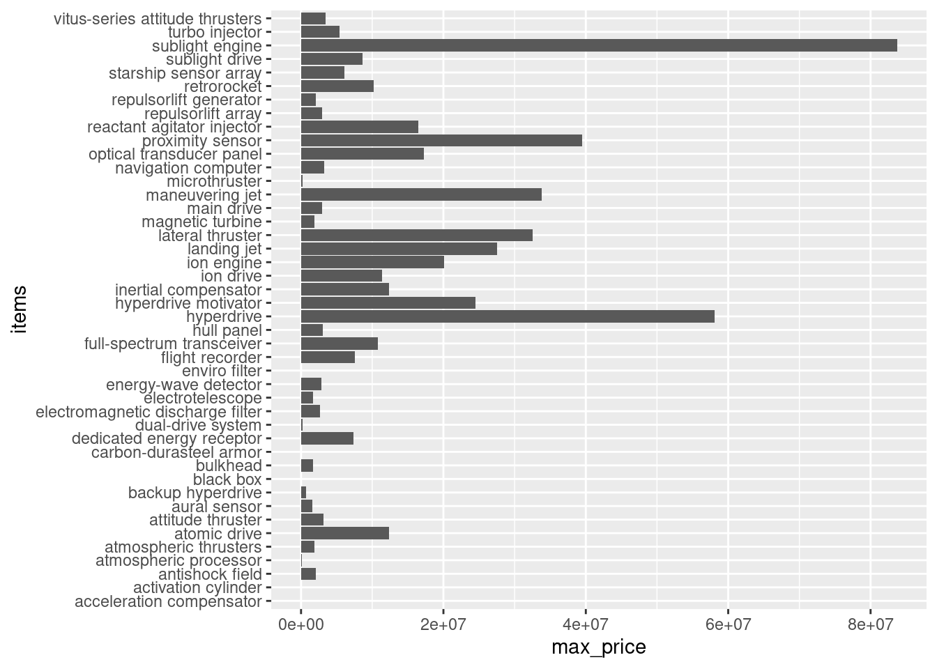
This plot might look better if the columns were sorted by their values.
Try reorder() to make this chart way more readable. Type “?reorder” to learn more about that function.
Show solution
ggplot(data = summary_scrap, aes(reorder(items, max_price), max_price)) +
  geom_col() +
  coord_flip()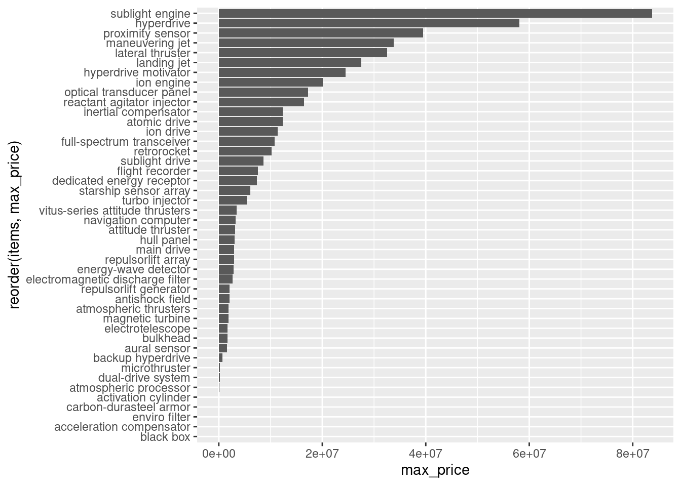
Nice work!! You may now move on to the Commodore level analysis.
