1 Day 1 review
Get to know your DATA
| Function | Information |
|---|---|
names(scrap) |
column names |
nrow(...) |
number of rows |
ncol(...) |
number of columns |
summary(...) |
summary of all column values (ex. max, mean, median) |
glimpse(...) |
column names + a glimpse of first values (requires dplyr package) |
Filtering
Menu of comparisons
Symbol Comparison >greater than >=greater than or equal to <less than <=less than or equal to ==equal to !=NOT equal to %in%value is in list: X %in% c(1,3,7)is.na(...)is the value missing? str_detect(col_name, "word")“word” appears in text?
Your analysis toolbox
dplyr is the hero for most analysis tasks. With these six functions you can accomplish just about anything you want with your data.
| Function | Job |
|---|---|
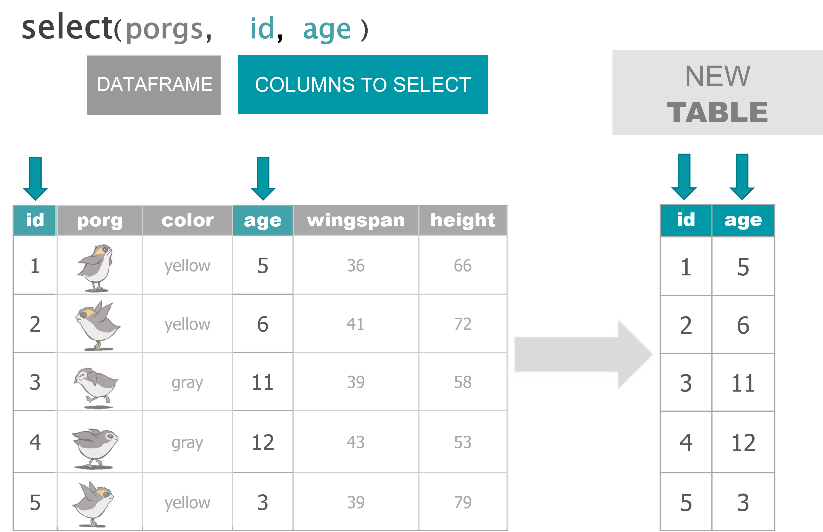
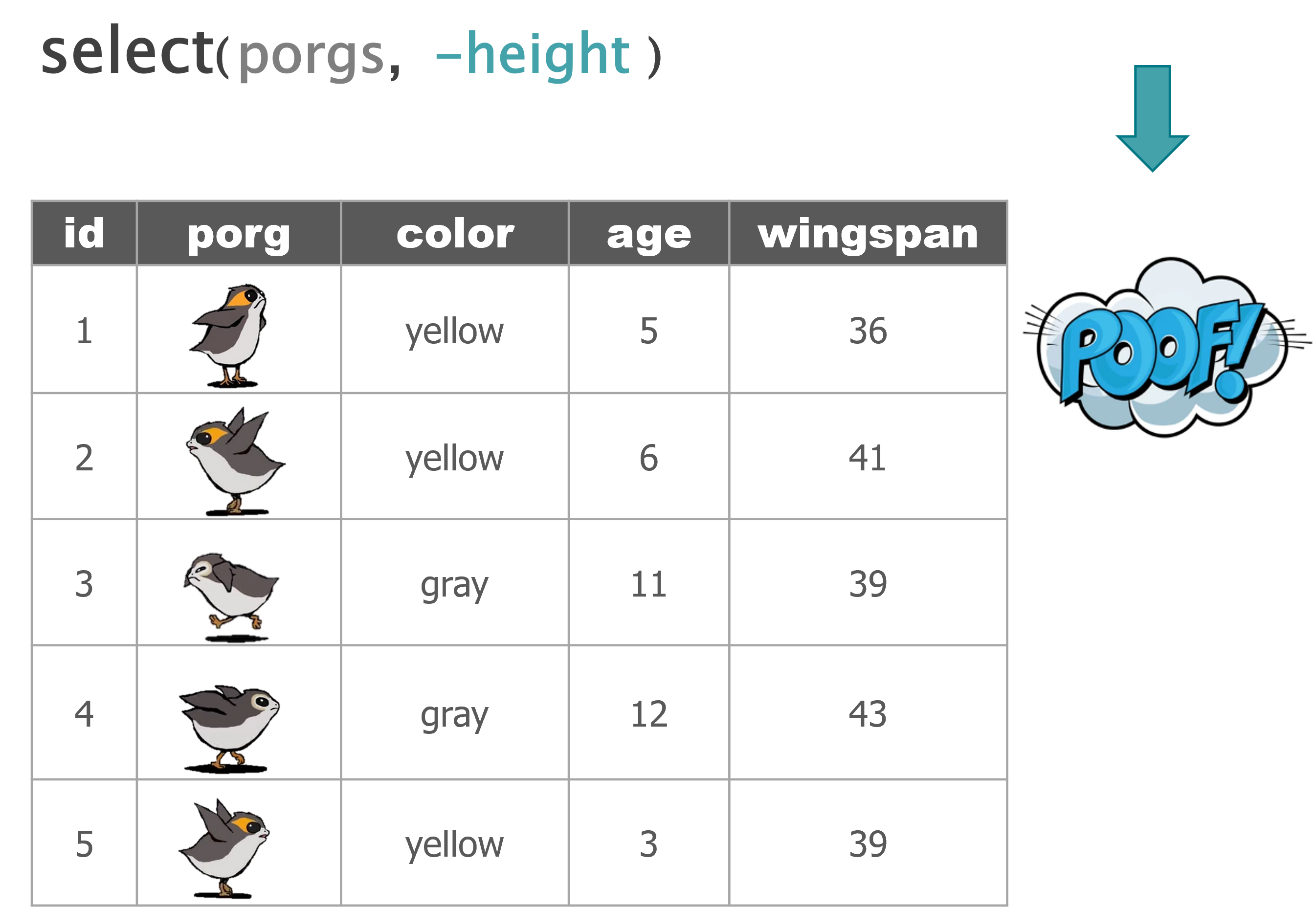
select() |
Select individual columns to drop or keep |
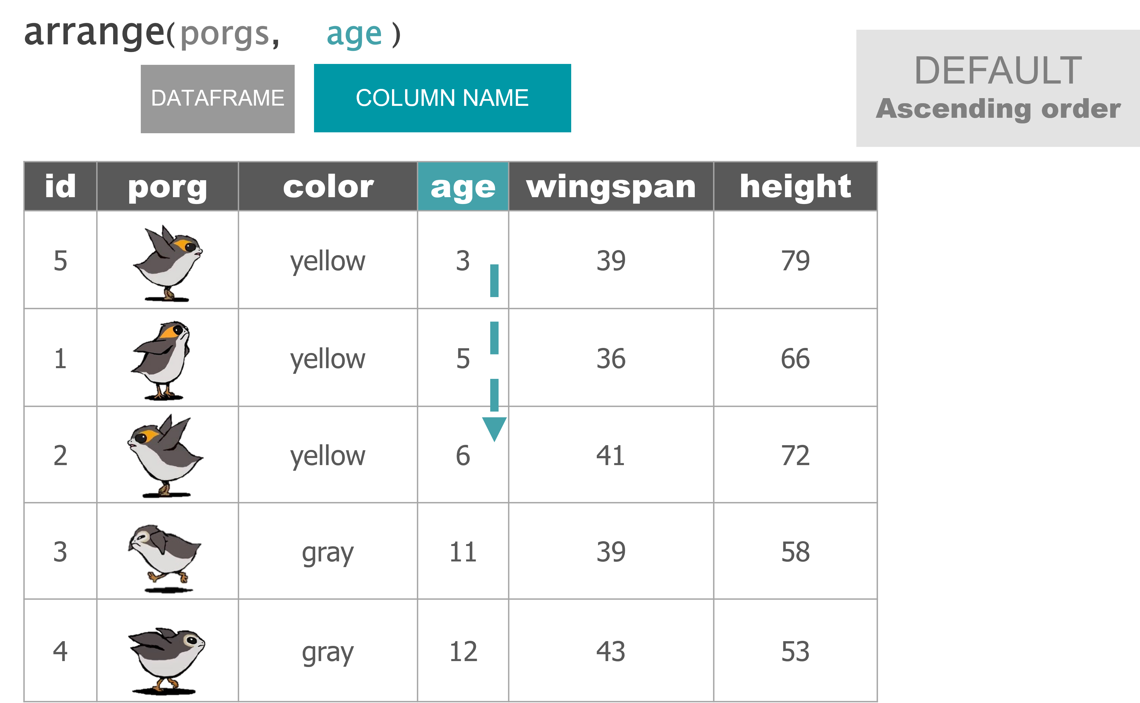
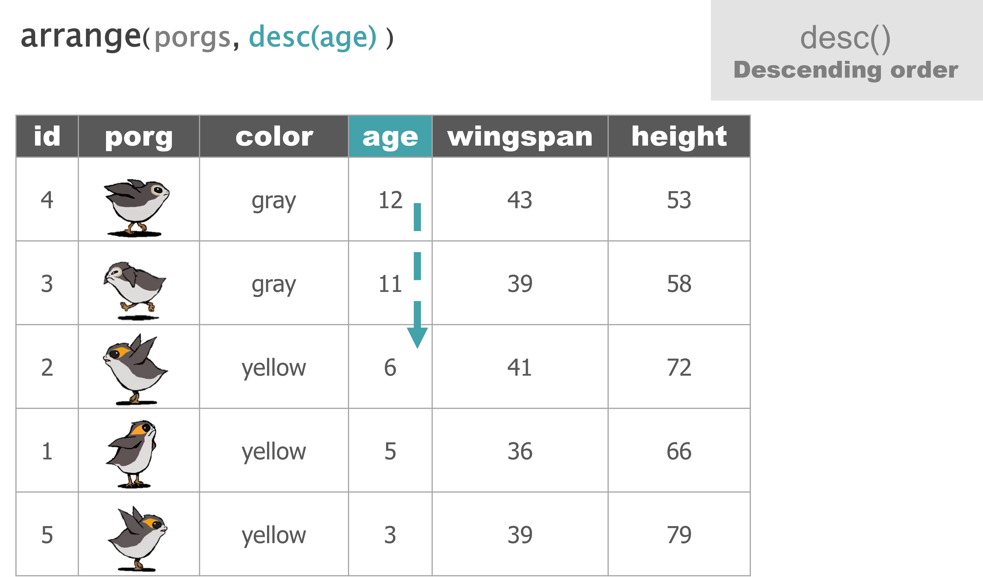
arrange() |
Sort a table top-to-bottom based on the values of a column |
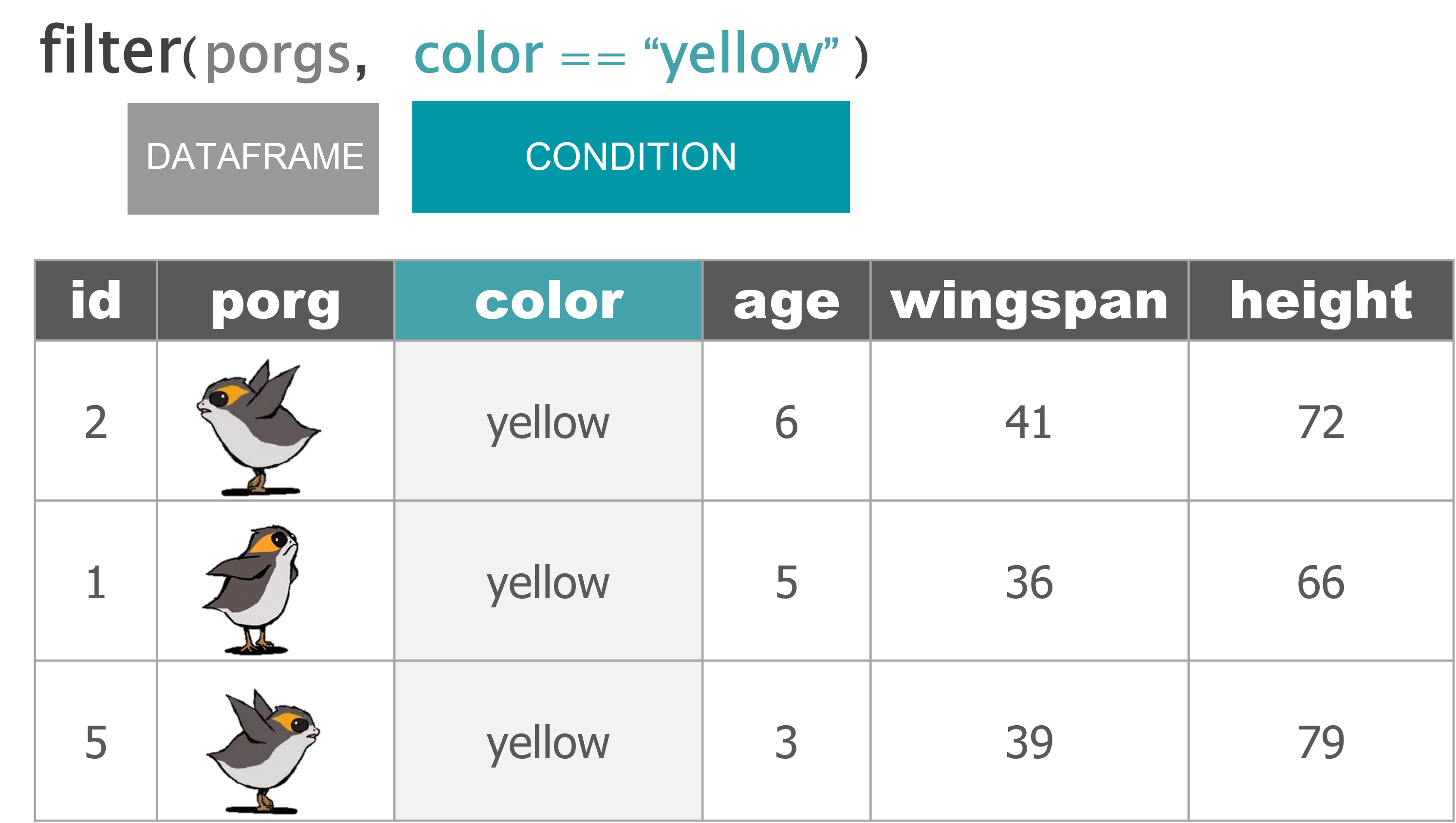
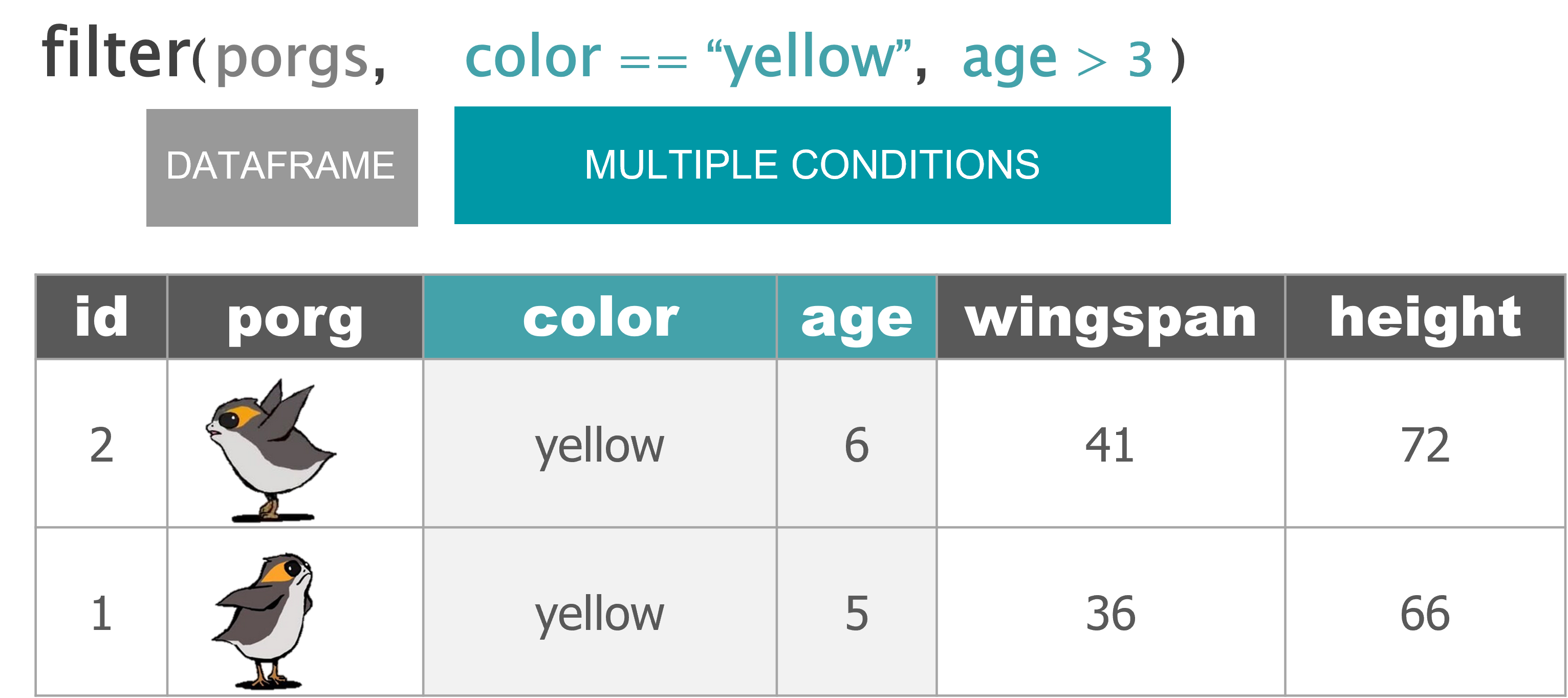
filter() |
Keep only a subset of rows depending on the values of a column |
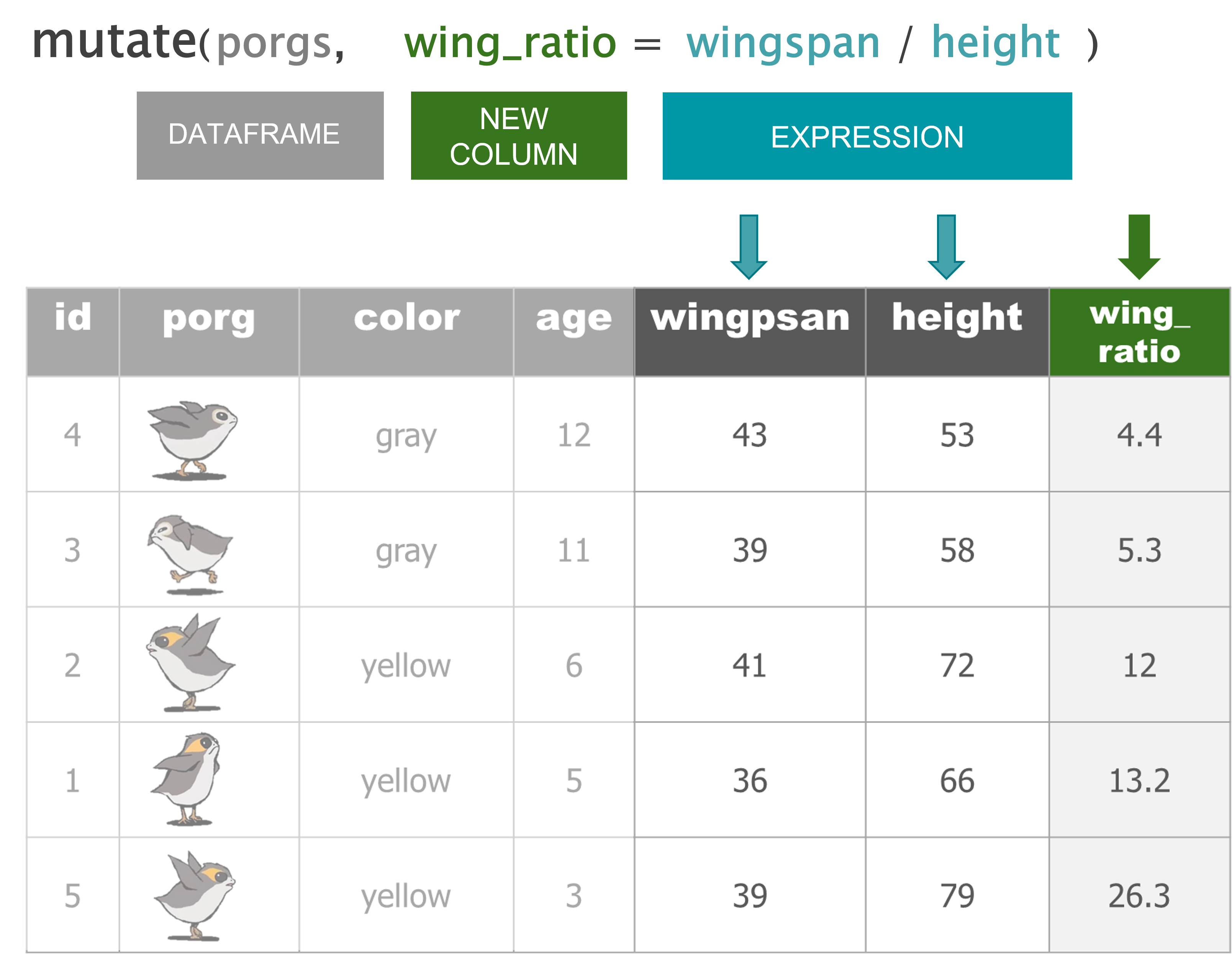
mutate() |
Add new columns or update existing columns |
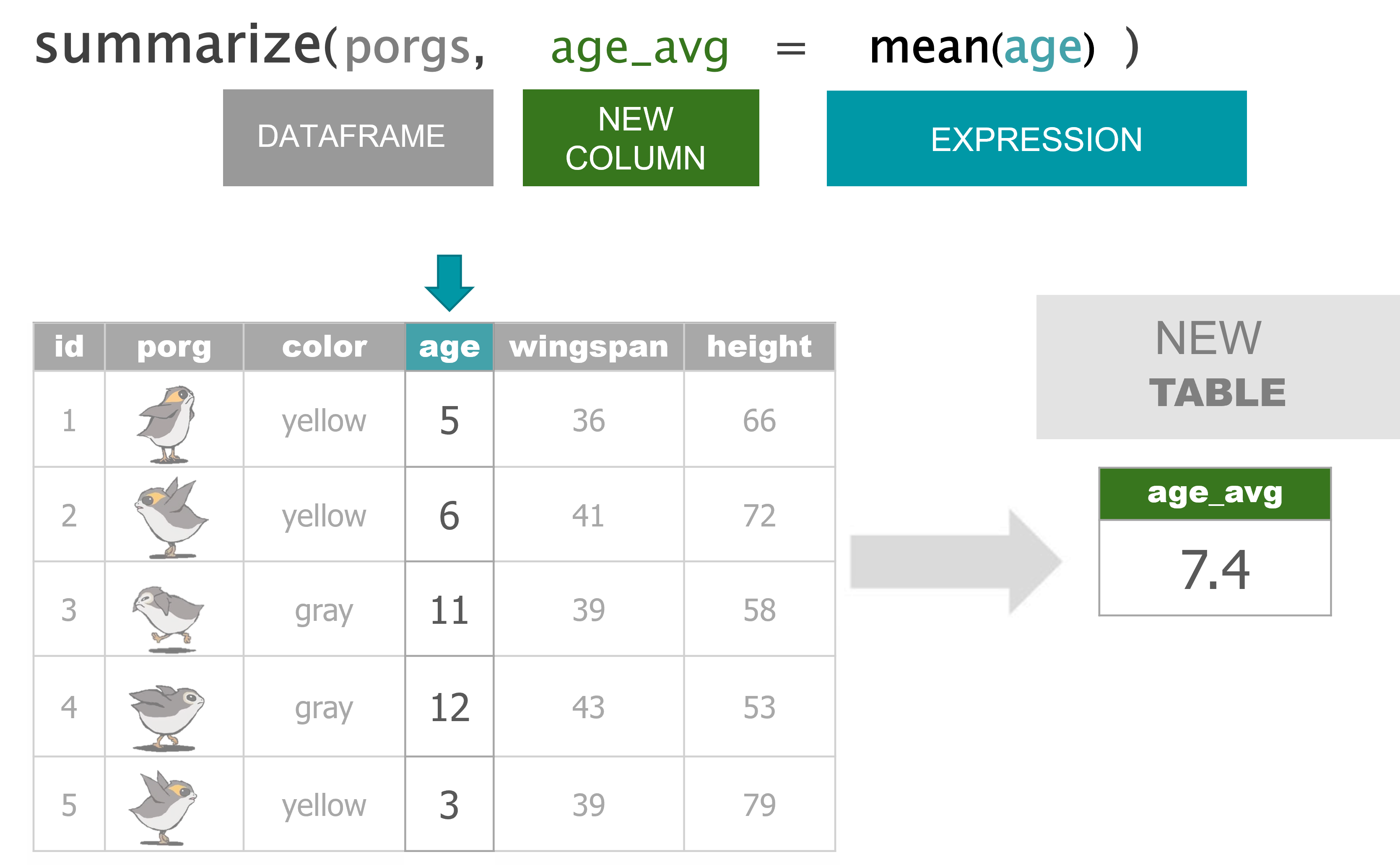
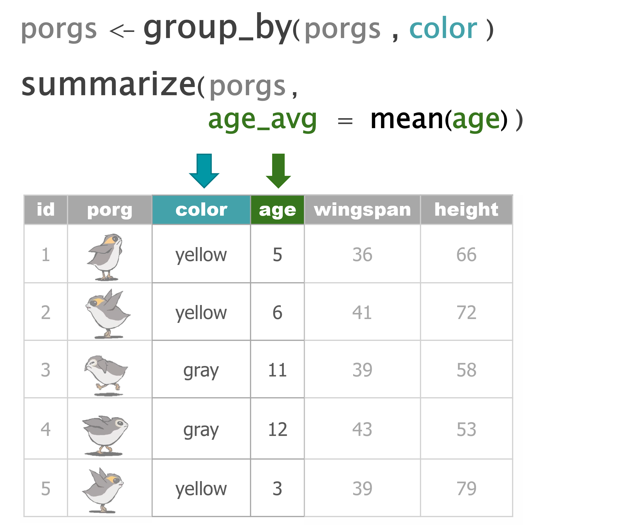
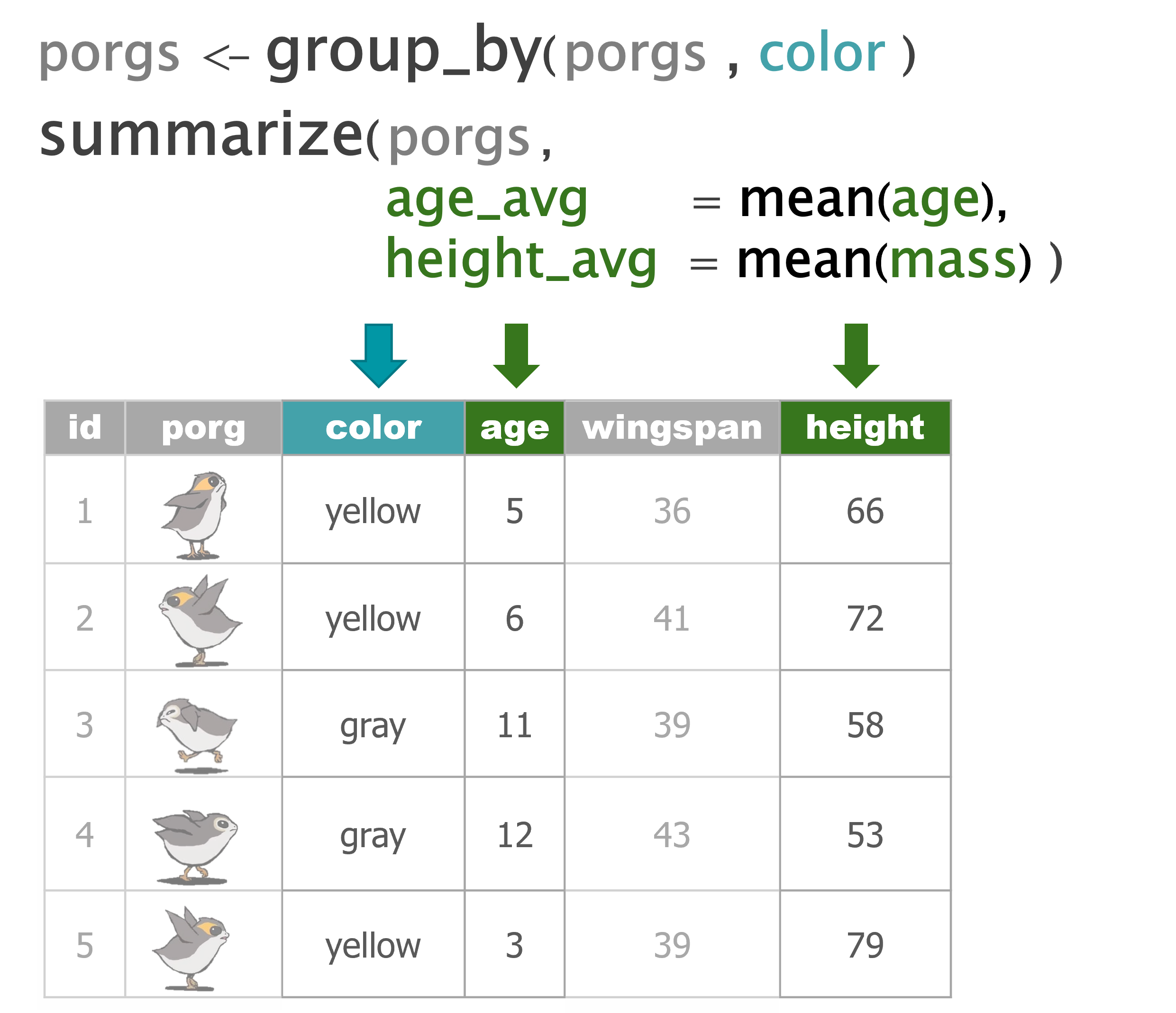
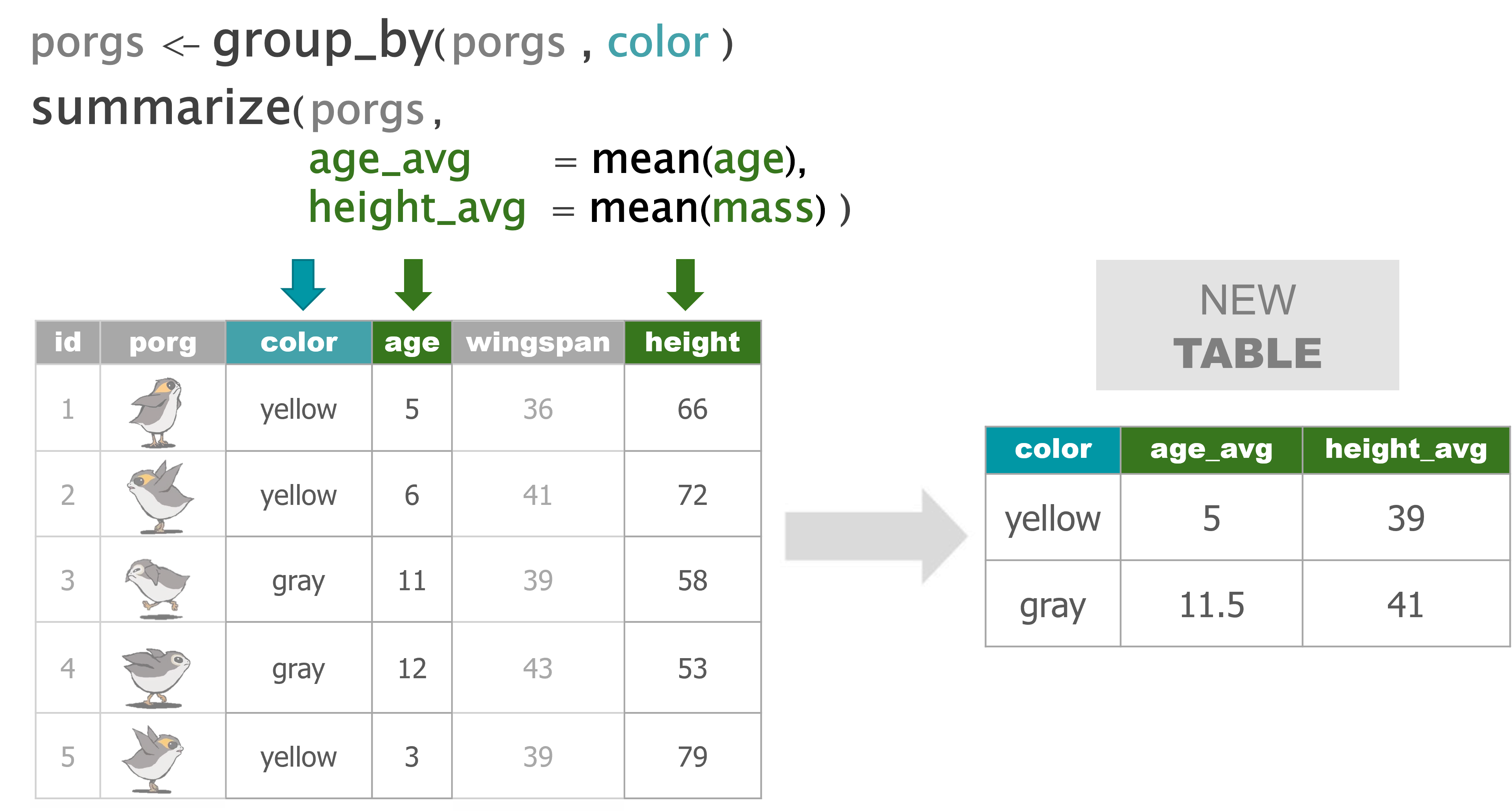
summarize() |
Calculate a single summary for an entire table |
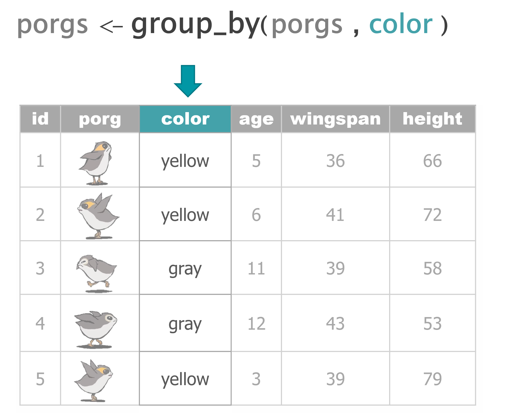
group_by() |
Sort data into groups based on the values of a column |
2 Day 2 review
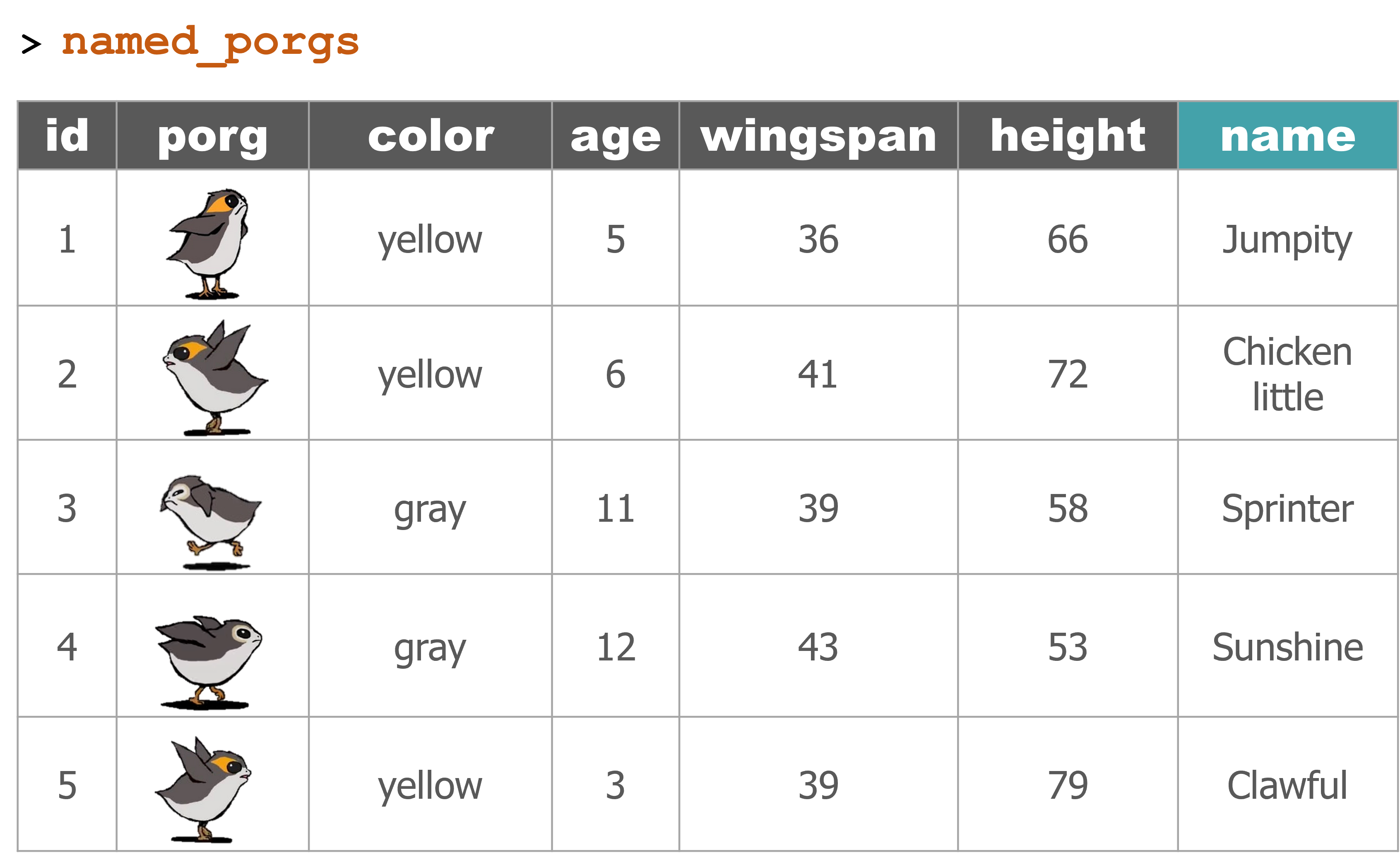
- Join tables with
left_join() summarize()functions- Group by category with
group_by() ifelse(): if THIS IS TRUE do a thing, otherwise do a different thing- Plots and charts with
ggplot
library(tidyverse)

porgs <- read_csv("https://mn-r.netlify.com/data/porg_data.csv")
porg_names <- read_csv("https://mn-r.netlify.com/data/porg_names.csv")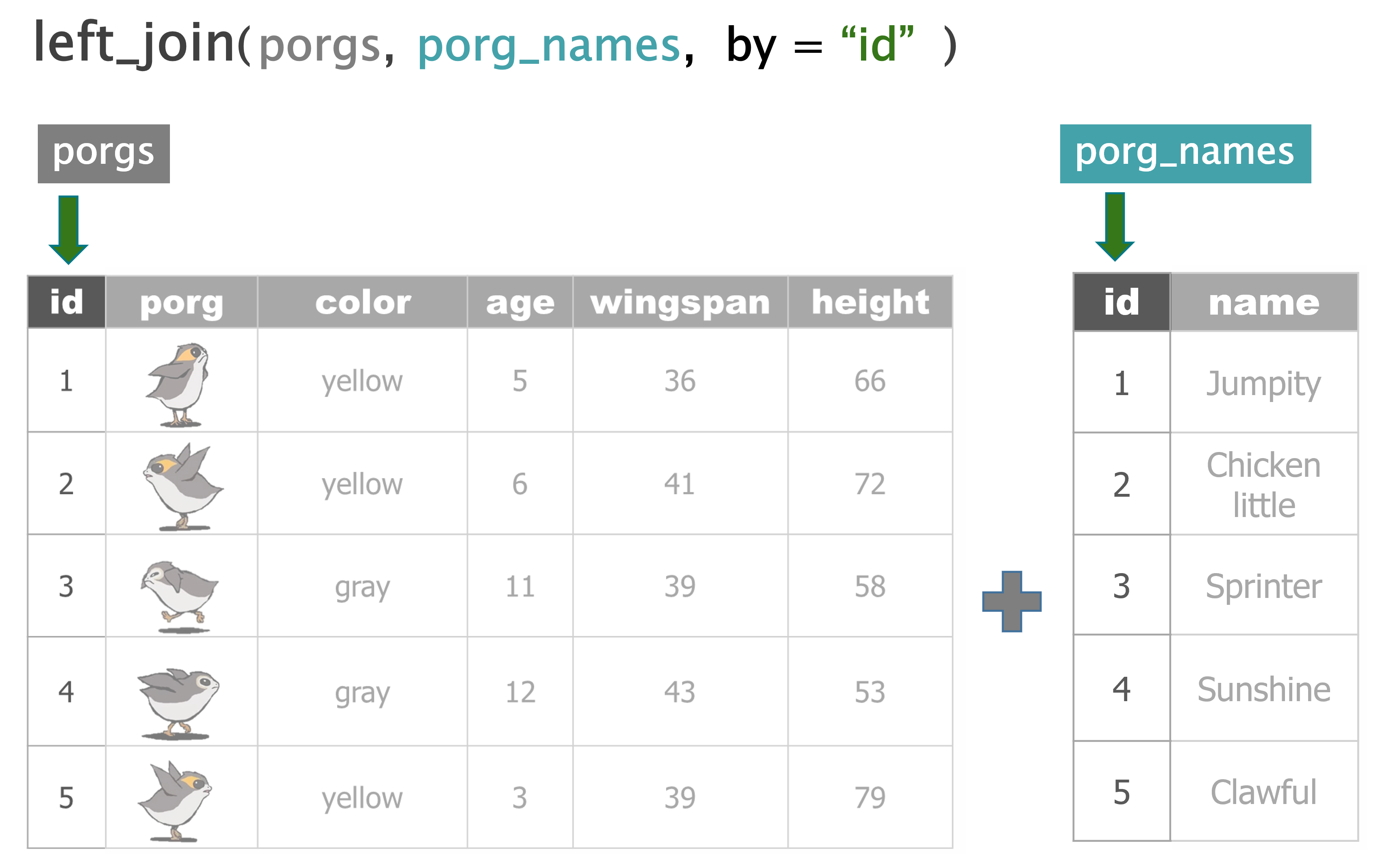
Welcome to Endor!

But wait…
The Ewoks say it’s unsafe to land. Not good. It sounds like the Empire is checking all incoming ships for licenses.
Lucky for us, there is some good news. The Ewoks say for a small ship like ours, it could be possible to land undetected. But we’ll have to put down right-dab in the middle of the 3 northern outposts.
Are you up for a challenge data droid?
Either way, let’s make a map to see what we’re up against. To help, our comrades sent along the coordinates of the Empire’s outposts. Guess what the first step is? That’s right. Time to add a new package.
3 Reading coordinates
To read coordinates stored in a CSV or Excel spreadsheet, we can read them into R with our usual friends:
- readr’s
read_csv()for CSV files - readxl’s
read_excel()for Excel files
For shapefiles, we use the sf package:
- sf’s
st_read()for SHP files
Get the coordinates from CSV
Take a look inside
## # A tibble: 3 × 3
##   ID      lat  long
##   <chr> <dbl> <dbl>
## 1 1NO    36.7 -119.
## 2 1NL    36.6 -119.
## 3 3NB 36.6 -119.## Rows: 3
## Columns: 3
## $ ID <chr> "1NO", "1NL", "3NB"
## $ lat <dbl> 36.65520, 36.58375, 36.59790
## $ long <dbl> -118.8469, -118.8195, -118.9022To make a quick map, use ggplot and add + geom_point().
library(ggplot2)

ggplot(outposts, aes(x = long, y = lat)) +
geom_point(size = 8, color = "steelblue") 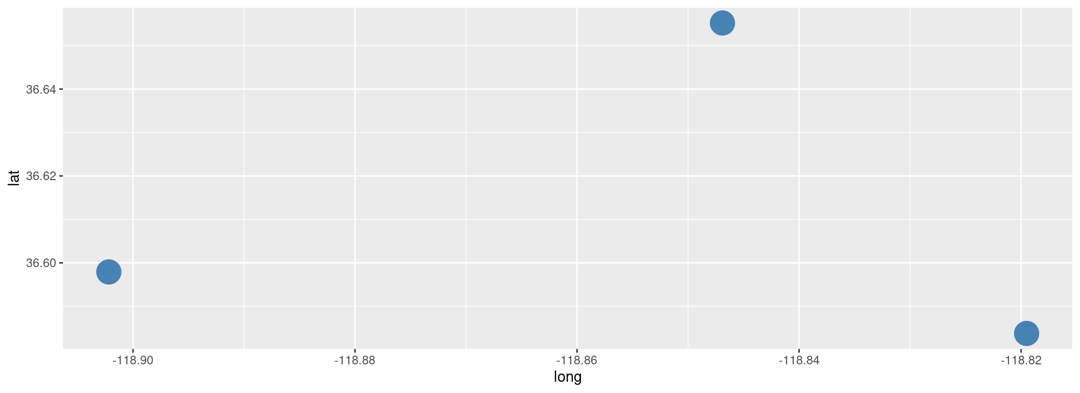
Where’s the center point?
Hint: How would you find the halfway point between two points?
Let’s use mutate() from the dplyr toolbox to update our location columns.
- Set the new
latcolumn to the center of all thelat’s - Set the new
longcolumn to the center of all thelong’s.
These will be the coordinates for our landing pad.
mutate the center
Complete the code
We found it!
Let’s add it to our map.
library(ggplot2)

ggplot(outposts, aes(x = long, y = lat)) +
  geom_point(size = 8, color = "steelblue") +
  geom_point(data = land_pad,
             aes(x = long, y = lat),
             size = 12,
             color = "green")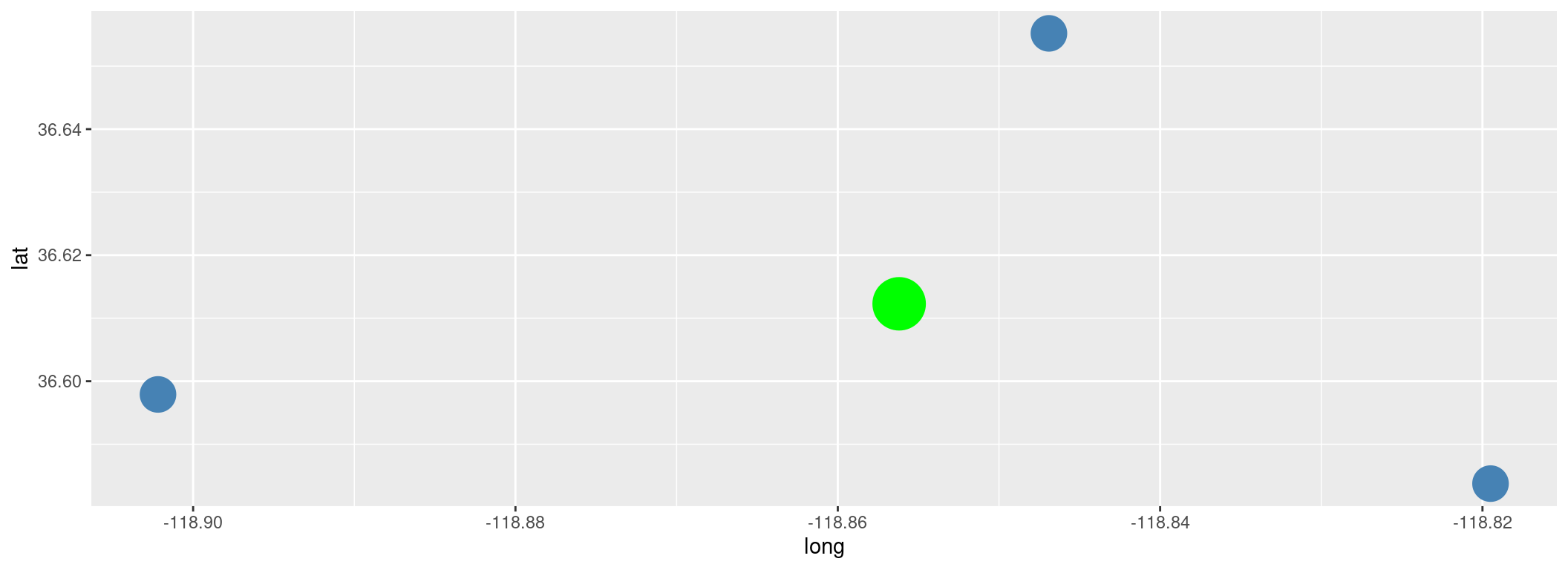
That’s looking good, but…
We’re going to need to be very precise to land perfectly in between these outposts. To make our captain really happy, let’s put this all in an interactive zoomable map. For interactive maps we use leaflet.
4 Leaflet maps
The leaflet package.

Leaflet makes interactive maps easy and you build them up in layers similar to a ggplot.
Maps that zoom
Leaflet builds map with layers similar to ggplot, but instead of adding things with the +, leaflet adds new layers with the %>% (“the pipe”).
1. Start with the outpost coordinates
2. Add the landing site
Fingers crossed it’s in the middle….
3. Add labels
Try hovering over one of the outposts to see its label.
leaflet(outposts) %>%
  addCircles(radius = 300,
             label = ~ID) %>%   #<<
  addTiles() %>%
  addMarkers(data  = land_pad,
             label = "Land HERE!",  #<<
             labelOptions = labelOptions(noHide = TRUE))  #<<
Explore!
News just came in that the outposts will soon be upgrading their radar to detect ships up to 4,200 meters away. Will that be a problem?
Steps
- Update the radius argument in
addCircles(...)to be equal to4200. - Add the argument
, fillColor = "yellow"insideaddCircles(..)
Show code
leaflet(outposts) %>%
  addCircles(radius = 4200, #<<
             label = ~ID,
             fillColor = "yellow") %>%
  addTiles() %>%
  addMarkers(data  = land_pad,
             label = "Land HERE!",
             labelOptions = labelOptions(noHide = TRUE))
Will our landing spot still be safe?
Woah! That’s a close one.
Great work data droid. Let’s take a minute to cool down…
Ok, now let’s land on that planet before we get stuck up here with permanent space legs.
BASEMAPS

There are lots of options for basemaps in leaflet. One of my favorites is CartoDB.Positron because its greyness doesn’t distract from the data.
Add it to your map by swapping out addTiles() for addProviderTiles(providers$CartoDB.Positron)
Show code
leaflet(outposts) %>%
  addCircles(radius = 4200,
             label = ~ID,
             fillColor = "yellow") %>%
   addProviderTiles(providers$CartoDB.Positron) %>%  #<<
   addMarkers(data  = land_pad,
              label = "Land HERE!",
              labelOptions = labelOptions(noHide = TRUE))
See more available basemaps at rstudio.github.io/leaflet/basemaps.
For more Leaflet examples, see the Full Leaflet Guide!
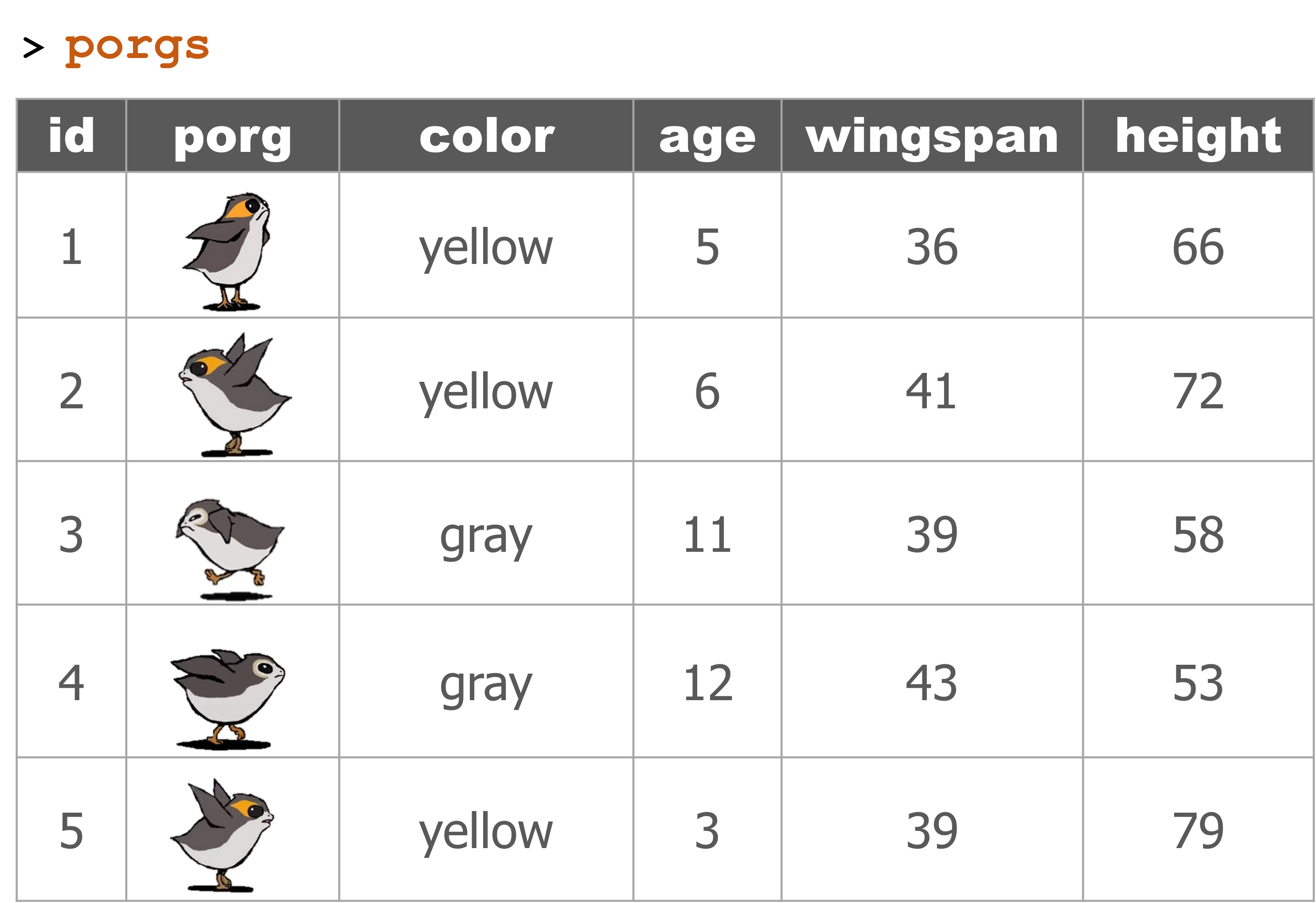
5 Invasive Porg Survey - 2023
The Ewoks need our help. There’s porgs EVERYWHERE!

Porgs have been spreading across the galaxy; likely by hitching rides on unsuspecting ships. They’re so cute people hate to say it, but they are starting to become a nuisance.
To get a grasp on the population explosion the Ewoks are launching a porg survey. And they need your help.
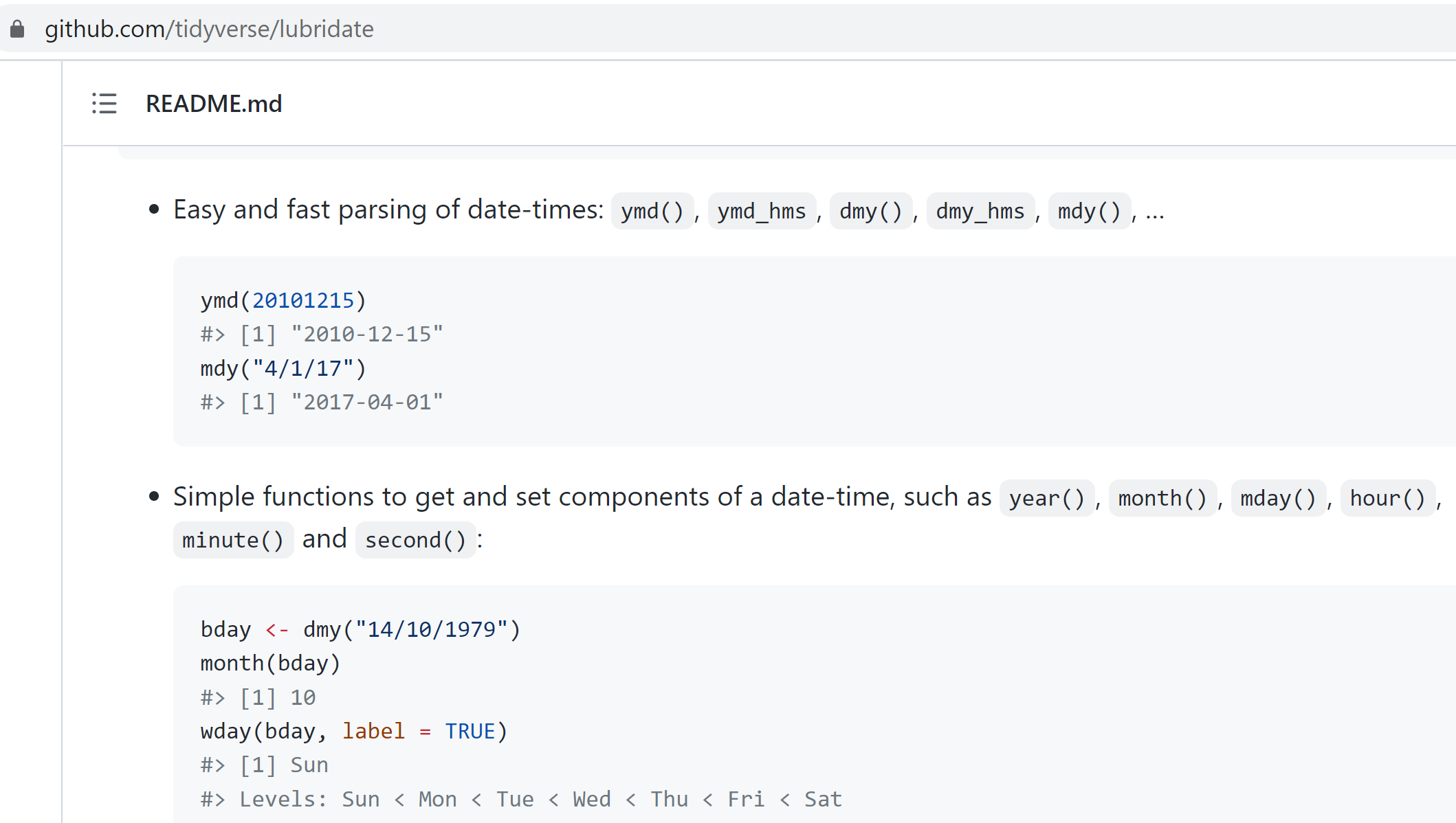
6 Dates with lubridate
The lubridate package.

It’s about time! Lubridate makes working with dates much easier.
We can find how much time has elapsed, add or subtract days, and find seasonal and day of the week averages. The package is included in the tidyverse bundle of packages, so it’s already installed!
View the date cheatsheet HERE.
It’s a great reference when you need to manipulate dates or timezones in your data.
1. Scheduling weekdays
![]()
Ewoks are very busy. They only have one day per week when they can volunteer.
Here is the weekday when volunteers are available at each location:
- Bright Tree:
Thursdays - Fern Gully:
Fridays
We can use the seq.Date() function and the option to step by = "week" to
generate the survey dates for each site. But we need to know which day to start from.
When is the first Thursday in May of 2023?
For that, we can use the wday(), the “weekday” function.
# wday tells you the day of week (Sun, Mon, etc..) for a specific date
wday(ymd('2023-05-01'), label = TRUE, abbr = FALSE)
## [1] Monday
## 7 Levels: Sunday < Monday < Tuesday < Wednesday < Thursday < ... < SaturdaySo the 1st of May will be a Monday.
That means…. May the 4th will be a Thursday. Perfect! That’s my favorite day.
Mutate to the rescue
We really don’t want to check every date one by one do we?
Let’s add a new week_day column to our survey table that checks ALL the dates ALL at once. To add a new column we call our friend mutate().
Complete the code below to add a week_day column.
filter() week days
With filter we can pick out only the days of the week that we want.
Split the schedule in two by filtering the survey to only the week day needed at each site:
Thursdayfor Bright TreeFridayfor Fern Gully
bright_dates <- filter(survey, week_day ==  ________ )

fern_dates   <- filter(survey, week_day ==  ________ )
Show code
How many survey dates are at each site?
Hint: It’s less than 50.
Show answer
26 survey days
2. Particular date formats

Oh no! Each survey site has a very-very particular Assistant to the Regional Manager. And they are demanding a very specific date format for their work schedules.
Before you send off the survey dates, you’ll need to adjust the dates to match the requested formats below.
Preferred date formats
- Bright Tree:
5-11-2023 - Fern Gully:
May 12, 2023
Use format(count_date, ...) and the date expressions below to format the schedule for each region accordingly.
For example:
format(count_date, "%b, %Y")prints the date asAug, 2023.
%bstands for 3-letter month abbreviation%Y%stands for the full 4 digit year
Date parts
| Expression | Description | Example |
|---|---|---|
%Y |
Year (4 digit) | 2023 |
%y |
Year (2 digit) | 21 |
%B |
Month (full name) | December |
%b |
Month (abbreviated) | Dec |
%m |
Month (decimal number) | 12 |
%d |
Day of the month (decimal number) | 30 |
Time parts
| Expression | Description | Example |
|---|---|---|
%H |
Hour | 8 |
%M |
Minute | 13 |
%S |
Second | 35 |
Use mutate() to update the week_day column in both site schedules.
Here’s a start
How’d we do?
| count_date | week_day | pretty_date |
|---|---|---|
| 2023-05-04 | Thursday | 05-04-2023 |
| 2023-05-11 | Thursday | 05-11-2023 |
| 2023-05-18 | Thursday | 05-18-2023 |
| count_date | week_day | pretty_date |
|---|---|---|
| 2023-05-05 | Friday | May 05, 2023 |
| 2023-05-12 | Friday | May 12, 2023 |
| 2023-05-19 | Friday | May 19, 2023 |
Congrats!
Your fine-tuned schedules worked perfectly.
Now let’s jump ahead and take a look at the survey results.
3. Results

Load the porg survey results.
Explore a bit.
Are there missing values?
A missing site
It looks like we have a slight missing data problem.
There’s a data point in the results that wasn’t labeled with the site location. We do know the date however.
On 2023-06-30 there were a whopping 7 porgs counted - but we just don’t know where.
Can you determine the site based on the date of the porg count?
Hint: What weekday is this?
Try the
wday(date)function.
Good sleuthing data droid.
We’ll learn how to update the site value later today, but right now we’re in a hurry, so let’s remove the row using filter.
Use filter() to keep only the rows in the porgs data where site is NOT NA (missing).
4. The best time for porgs
What is the best month to see porgs?
First, add a month column to the data with the function month() and the column count_date.
Next, use ggplot() and geom_col() to plot the porg sightings by month.
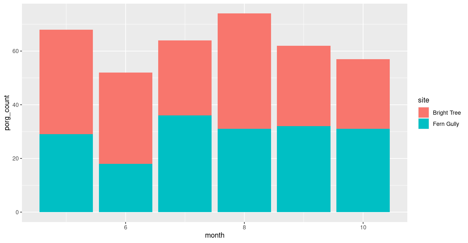
Why might June be the lowest month?
Hint: Fern Gully
5. Time series: All the data
Plot all the data with geom_point(). Put count_date on the x-axis, and the porg_count on the y-axis. Set the color to match the site column.
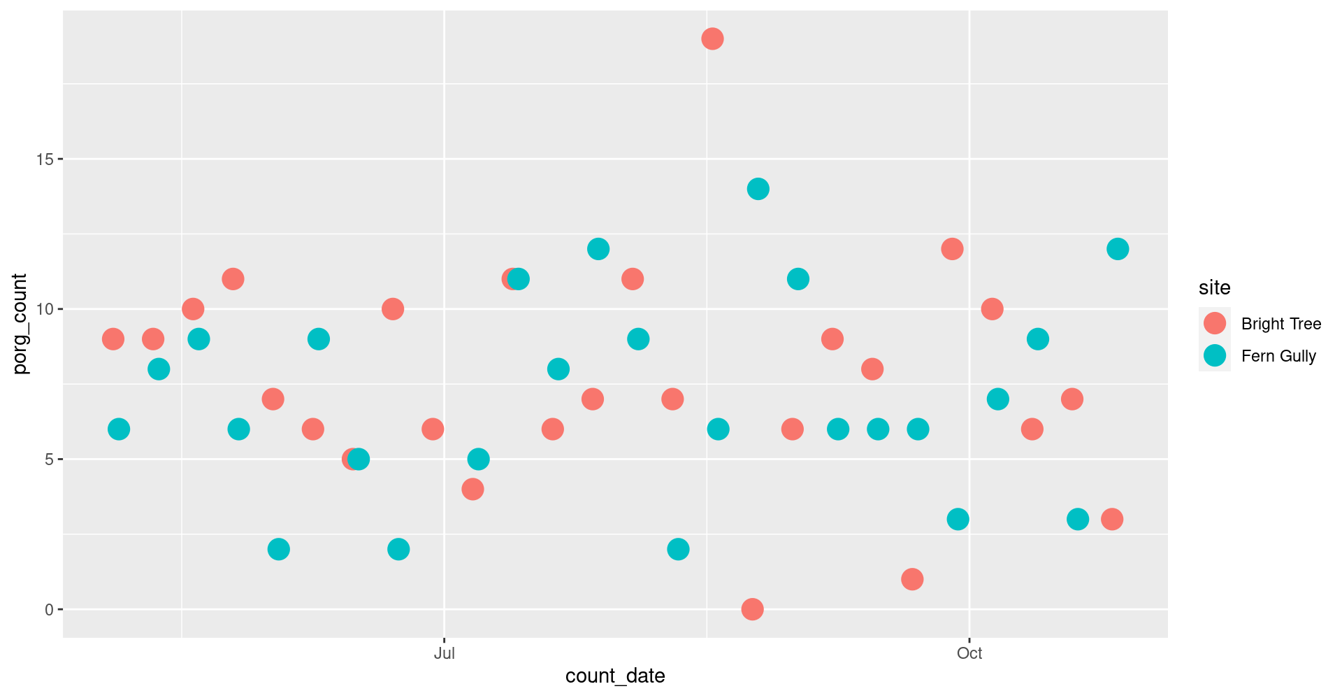
Oof! That’s a busy plot. Try adding + facet_wrap("site") to the end.
What happens?
ggplot(porgs, aes(x = count_date, y = porg_count, color = site)) +
geom_point(size = 5) +
facet_wrap("site") #<<Try adding + geom_line().
ggplot(porgs, aes(x = count_date, y = porg_count, color = site)) +
  geom_point(size = 5) +
  facet_wrap(~ site) +
  geom_line()                #<<
Show code
ggplot(porgs, aes(x = count_date, y = porg_count, color = site)) +
  geom_point(size = 5) +
  facet_wrap(~ site) +
  geom_line()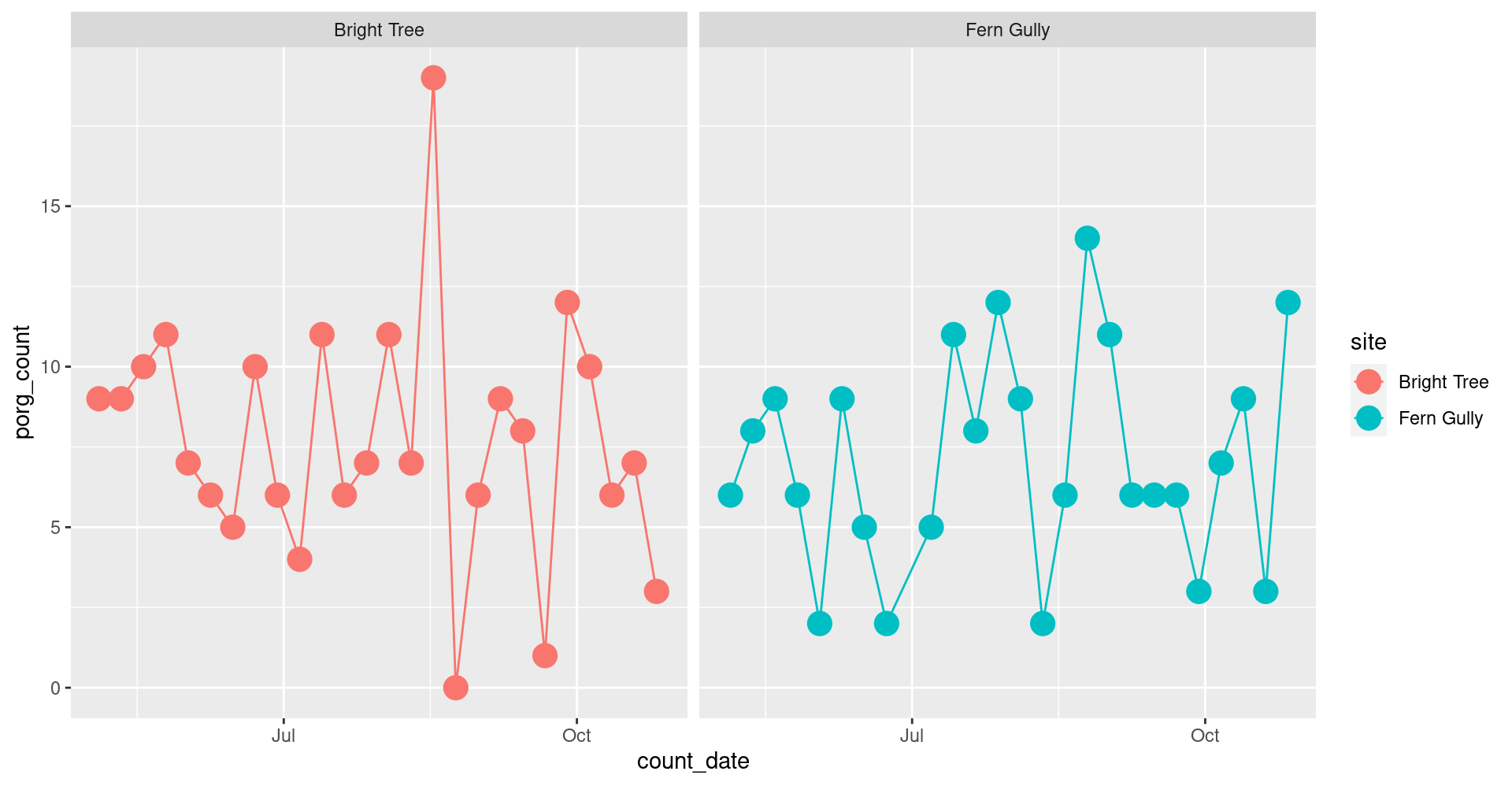
Great work
The Ewoks are deeply thankful. They’ll be in touch for Porg Survey 2024.

7 Share with friends

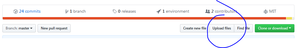
Add a new repository
Now we can create a new repository to store some of our new R plots and scripts. Click the bright green New button to get started.

- Give it a short name like
Rplots - Keep it public
- Check the box to initialize with a README
- Click
[ Create repository ]
Add an R script or plot
Click Upload files to add an image of an R plot or one of your .R scripts.
Package questions
Google: "package name" + github
For example, here’s the top page for lubridate + github